Recap
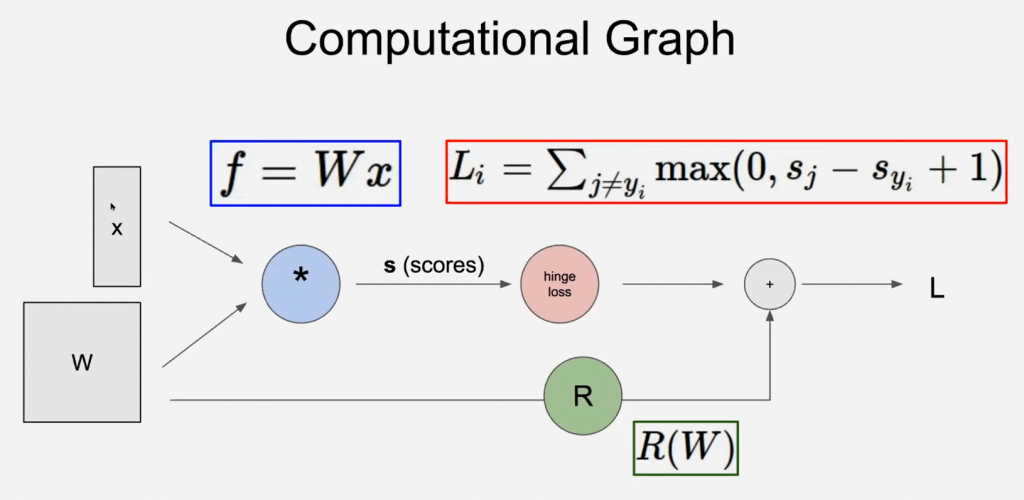
- We have a score function: $s=f(x ; W) \stackrel{\text { e.g. }}{=} W x$
- We have a loss function:
- Softmax: $L_{i}=-\log \left(\frac{e^{e y_{i}}}{\sum_{j} e^{s_{j}}}\right)$
- SVM: $L_{i}=\sum_{j \neq y_{i}} \max \left(0, s_{j}-s_{y_{i}}+1\right)$
- Thus, the Full loss $L=\frac{1}{N} \sum_{i=1}^{N} L_{i}+R(W)$
$R(W)–\lambda R(W)$ control the strenth of regularization penalty. 当这个增大的时候会得到一个smoother的boundry, basically by limiting the flexibility of the W matrix. 让W不要太有灵活性,灵活性太高就容易过拟合训练集。训练过程就是捏神经网络形状让它拟合训练数据的过程,就像捏橡皮泥,不能太像训练数据了,会没有泛化能力。控制正则项的梯度反向传播程度。
Gradient descent
- Numerical gradient: approximate, slow, easy to write
- Analytic gradient: exact, fast, error-prone
In practice, we always use analytic gradient, but we check implementation with numerical gradient. This is called a gradient check.
Mini-batch Gradient Descent
Only use a small portion of the training set to compute the gradient. (with random subsets)
It just like sampling, since the loss function will give the average loss for data loss.
- Goal is to estimate the gradient
- Trade-off between accu and compu
- No point in doing more computation if it wont change the updates
We take one step according to one sample and update the $W$ once. Then we catch another sample with a constant size of batch, take step, update $W$. Each time we may do harm to some data but in average, the loss is reducing.
Computational Graph
